r travel time

travel_time_matrix: Calculate travel time matrix between origin destination pairs

Description.

Fast computation of travel time estimates between one or multiple origin destination pairs.

A data.table with travel time estimates (in minutes) between origin and destination pairs. Pairs whose trips couldn't be completed within the maximum travel time and/or whose origin is too far from the street network are not returned in the data.table . If output_dir is not NULL , the function returns the path specified in that parameter, in which the .csv files containing the results are saved.

An object to connect with the R5 routing engine, created with setup_r5() .

Either a POINT sf object with WGS84 CRS, or a data.frame containing the columns id , lon and lat .

A character vector. The transport modes allowed for access, transfer and vehicle legs of the trips. Defaults to WALK . Please see details for other options.

A character vector. The transport mode used after egress from the last public transport. It can be either WALK , BICYCLE or CAR . Defaults to WALK . Ignored when public transport is not used.

A POSIXct object. Please note that the departure time only influences public transport legs. When working with public transport networks, please check the calendar.txt within your GTFS feeds for valid dates. Please see details for further information on how datetimes are parsed.

An integer. The time window in minutes for which r5r will calculate multiple travel time matrices departing each minute. Defaults to 10 minutes. By default, the function returns the result based on median travel times, but the user can set the percentiles parameter to extract more results. Please read the time window vignette for more details on its usage vignette("time_window", package = "r5r")

An integer vector (max length of 5). Specifies the percentile to use when returning travel time estimates within the given time window. For example, if the 25th travel time percentile between A and B is 15 minutes, 25% of all trips taken between these points within the specified time window are shorter than 15 minutes. Defaults to 50, returning the median travel time. If a vector with length bigger than 1 is passed, the output contains an additional column for each percentile specifying the percentile travel time estimate. each estimate. Due to upstream restrictions, only 5 percentiles can be specified at a time. For more details, please see R5 documentation at https://docs.conveyal.com/analysis/methodology#accounting-for-variability .

A fare structure object, following the convention set in setup_fare_structure() . This object describes how transit fares should be calculated. Please see the fare structure vignette to understand how this object is structured: vignette("fare_structure", package = "r5r") .

A number. The maximum value that trips can cost when calculating the fastest journey between each origin and destination pair.

An integer. The maximum walking time (in minutes) to access and egress the transit network, to make transfers within the network or to complete walk-only trips. Defaults to no restrictions (numeric value of Inf ), as long as max_trip_duration is respected. When routing transit trips, the max time is considered separately for each leg (e.g. if you set max_walk_time to 15, you could get trips with an up to 15 minutes walk leg to reach transit and another up to 15 minutes walk leg to reach the destination after leaving transit. In walk-only trips, whenever max_walk_time differs from max_trip_duration , the lowest value is considered.

An integer. The maximum cycling time (in minutes) to access and egress the transit network, to make transfers within the network or to complete bicycle-only trips. Defaults to no restrictions (numeric value of Inf ), as long as max_trip_duration is respected. When routing transit trips, the max time is considered separately for each leg (e.g. if you set max_bike_time to 15, you could get trips with an up to 15 minutes cycle leg to reach transit and another up to 15 minutes cycle leg to reach the destination after leaving transit. In bicycle-only trips, whenever max_bike_time differs from max_trip_duration , the lowest value is considered.

An integer. The maximum driving time (in minutes) to access and egress the transit network. Defaults to no restrictions, as long as max_trip_duration is respected. The max time is considered separately for each leg (e.g. if you set max_car_time to 15 minutes, you could potentially drive up to 15 minutes to reach transit, and up to another 15 minutes to reach the destination after leaving transit). Defaults to Inf , no limit.

An integer. The maximum trip duration in minutes. Defaults to 120 minutes (2 hours).

A numeric. Average walk speed in km/h. Defaults to 3.6 km/h.

A numeric. Average cycling speed in km/h. Defaults to 12 km/h.

An integer. The maximum number of public transport rides allowed in the same trip. Defaults to 3.

An integer between 1 and 4. The maximum level of traffic stress that cyclists will tolerate. A value of 1 means cyclists will only travel through the quietest streets, while a value of 4 indicates cyclists can travel through any road. Defaults to 2. Please see details for more information.

An integer. The number of Monte Carlo draws to perform per time window minute when calculating travel time matrices and when estimating accessibility. Defaults to 5. This would mean 300 draws in a 60-minute time window, for example. This parameter only affects the results when the GTFS feeds contain a frequencies.txt table.

An integer. The number of threads to use when running the router in parallel. Defaults to use all available threads (Inf).

A logical. Whether to show R5 informative messages when running the function. Defaults to FALSE (please note that in such case R5 error messages are still shown). Setting verbose to TRUE shows detailed output, which can be useful for debugging issues not caught by r5r .

A logical. Whether to show a progress counter when running the router. Defaults to FALSE . Only works when verbose is set to FALSE , so the progress counter does not interfere with R5 's output messages. Setting progress to TRUE may impose a small penalty for computation efficiency, because the progress counter must be synchronized among all active threads.

Either NULL or a path to an existing directory. When not NULL (the default), the function will write one .csv file with the results for each origin in the specified directory. In such case, the function returns the path specified in this parameter. This parameter is particularly useful when running on memory-constrained settings because writing the results directly to disk prevents r5r from loading them to RAM memory.

Transport modes

R5 allows for multiple combinations of transport modes. The options include:

Transit modes: TRAM , SUBWAY , RAIL , BUS , FERRY , CABLE_CAR , GONDOLA , FUNICULAR . The option TRANSIT automatically considers all public transport modes available.

Non transit modes: WALK , BICYCLE , CAR , BICYCLE_RENT , CAR_PARK .

Level of Traffic Stress (LTS)

When cycling is enabled in R5 (by passing the value BIKE to either mode or mode_egress ), setting max_lts will allow cycling only on streets with a given level of danger/stress. Setting max_lts to 1, for example, will allow cycling only on separated bicycle infrastructure or low-traffic streets and routing will revert to walking when traversing any links with LTS exceeding 1. Setting max_lts to 3 will allow cycling on links with LTS 1, 2 or 3. Routing also reverts to walking if the street segment is tagged as non-bikable in OSM (e.g. a staircase), independently of the specified max LTS.

The default methodology for assigning LTS values to network edges is based on commonly tagged attributes of OSM ways. See more info about LTS in the original documentation of R5 from Conveyal at https://docs.conveyal.com/learn-more/traffic-stress . In summary:

LTS 1 : Tolerable for children. This includes low-speed, low-volume streets, as well as those with separated bicycle facilities (such as parking-protected lanes or cycle tracks).

LTS 2 : Tolerable for the mainstream adult population. This includes streets where cyclists have dedicated lanes and only have to interact with traffic at formal crossing.

LTS 3 : Tolerable for "enthused and confident" cyclists. This includes streets which may involve close proximity to moderate- or high-speed vehicular traffic.

LTS 4 : Tolerable only for "strong and fearless" cyclists. This includes streets where cyclists are required to mix with moderate- to high-speed vehicular traffic.

For advanced users, you can provide custom LTS values by adding a tag <key = "lts"> to the osm.pbf file.

Datetime parsing

r5r ignores the timezone attribute of datetime objects when parsing dates and times, using the study area's timezone instead. For example, let's say you are running some calculations using Rio de Janeiro, Brazil, as your study area. The datetime as.POSIXct("13-05-2019 14:00:00", format = "%d-%m-%Y %H:%M:%S") will be parsed as May 13th, 2019, 14:00h in Rio's local time, as expected. But as.POSIXct("13-05-2019 14:00:00", format = "%d-%m-%Y %H:%M:%S", tz = "Europe/Paris") will also be parsed as the exact same date and time in Rio's local time, perhaps surprisingly, ignoring the timezone attribute.

Routing algorithm

The travel_time_matrix() , expanded_travel_time_matrix() and accessibility() functions use an R5 -specific extension to the RAPTOR routing algorithm (see Conway et al., 2017). This RAPTOR extension uses a systematic sample of one departure per minute over the time window set by the user in the 'time_window' parameter. A detailed description of base RAPTOR can be found in Delling et al (2015). However, whenever the user includes transit fares inputs to these functions, they automatically switch to use an R5 -specific extension to the McRAPTOR routing algorithm.

Conway, M. W., Byrd, A., & van der Linden, M. (2017). Evidence-based transit and land use sketch planning using interactive accessibility methods on combined schedule and headway-based networks. Transportation Research Record, 2653(1), 45-53. tools:::Rd_expr_doi("10.3141/2653-06")

Delling, D., Pajor, T., & Werneck, R. F. (2015). Round-based public transit routing. Transportation Science, 49(3), 591-604. tools:::Rd_expr_doi("10.1287/trsc.2014.0534")

Other routing: detailed_itineraries() , expanded_travel_time_matrix() , pareto_frontier()

Run the code above in your browser using DataLab

Navigation Menu

Search code, repositories, users, issues, pull requests..., provide feedback.

We read every piece of feedback, and take your input very seriously.

Saved searches

Use saved searches to filter your results more quickly.

To see all available qualifiers, see our documentation .

• Notifications

TravelTime SDK for R programming language

Licenses found

Traveltime-dev/traveltime-sdk-r, folders and files, repository files navigation, travel time r sdk.

Travel Time R SDK helps users find locations by journey time rather than using ‘as the crow flies’ distance. Time-based searching gives users more opportunities for personalisation and delivers a more relevant search.

Installation

You can install Travel Time R SDK hosted on CRAN repository with the following command:

System requirements

traveltimeR uses rprotobuf as a dependency. If your package installation fails, please make sure you have the system requirements covered for rprotobuf

Debian/Ubuntu

There also exists similar commands on other distributions or operating systems.

Authentication

In order to authenticate with Travel Time API, you will have to supply the Application ID and API Key.

Isochrones (Time Map)

Given origin coordinates, find shapes of zones reachable within corresponding travel time. Find unions/intersections between different searches.

Isochrones (Time Map) Fast

A very fast version of Isochrone API. However, the request parameters are much more limited.

Distance Map

Given origin coordinates, find shapes of zones reachable within corresponding travel distance. Find unions/intersections between different searches.

Distance Matrix (Time Filter)

Given origin and destination points filter out points that cannot be reached within specified time limit. Find out travel times, distances and costs between an origin and up to 2,000 destination points.

Body attributes:

• locations: Locations to use. Each location requires an id and lat/lng values.
• departure_searches: Searches based on departure times. Leave departure location at no earlier than given time. You can define a maximum of 10 searches.
• arrival_searches: Searches based on arrival times. Arrive at destination location at no later than given time. You can define a maximum of 10 searches.

Returns routing information between source and destinations.

Time Filter (Fast)

A very fast version of time_filter() . However, the request parameters are much more limited.

Time Filter Fast (Proto)

A fast version of time filter communicating using protocol buffers .

The request parameters are much more limited and only travel time is returned. In addition, the results are only approximately correct (95% of the results are guaranteed to be within 5% of the routes returned by regular time filter).

This inflexibility comes with a benefit of faster response times (Over 5x faster compared to regular time filter) and larger limits on the amount of destination points.

• departureLat: Origin point latitude.
• departureLng: Origin point longitude.
• destinationCoordinates: Destination points. Cannot be more than 200,000.
• transportation: Transportation type.
• travelTime: Time limit.
• country: Return the results that are within the specified country.

Time Filter (Postcode Districts)

Find reachable postcodes from origin (or to destination) and get statistics about such postcodes. Currently only supports United Kingdom.

Time Filter (Postcode Sectors)

Find sectors that have a certain coverage from origin (or to destination) and get statistics about postcodes within such sectors. Currently only supports United Kingdom.

Time Filter (Postcodes)

Geocoding (search).

Match a query string to geographic coordinates.

Function accepts the following parameters:

• query - A query to geocode. Can be an address, a postcode or a venue.
• within.country - Only return the results that are within the specified country or countries. If no results are found it will return the country itself. Optional. Format:ISO 3166-1 alpha-2 or alpha-3.
• format.exclude.country - Format the name field of the response to a well formatted, human-readable address of the location. Experimental. Optional.
• format.name - Exclude the country from the formatted name field (used only if format.name is equal true). Optional.
• bounds - Used to limit the results to a bounding box. Expecting a character vector with four floats, marking a south-east and north-west corners of a rectangle: min-latitude,min-longitude,max-latitude,max-longitude. e.g. bounds for Scandinavia c(54.16243,4.04297,71.18316,31.81641). Optional.

Reverse Geocoding

Attempt to match a latitude, longitude pair to an address.

• lat - Latitude of the point to reverse geocode.
• lng - lng Longitude of the point to reverse geocode.

Get information about currently supported countries.

Supported Locations

Find out what points are supported by the api.

Contributors 9

traveltime - a Traveltime API Wrapper for R

1 querying the traveltime-api with traveltime_map, 2 taking a glimpse at the isochrones (mapview), 3 plotting a traveltime-map (ggmap & ggplot2), 4 creating an animated map with gganimate : rush hour vs night time drive.

The traveltime-package allows to retrieve isochrones for traveltime-maps from the Traveltime Platform API directly from R. The isochrones are stored as sf-objects, ready for visualization or further processing. The isochrones display how far you can travel from a certain location within a given timeframe. Numerous modes of transport are supported.

http://docs.traveltimeplatform.com/overview/introduction

GET an API-KEY here: http://docs.traveltimeplatform.com/overview/getting-keys/

For non-commercial use the usage of the API is free up to 10’000 queries a month (max 30 queries per min). For commercial use (e.g. to integrate the API into a website) a license is needed.

You can easily retrieve the isochrones with the traveltime_map function. Find a list of supported countries here: http://docs.traveltimeplatform.com/overview/supported-countries/

If you are interested in the opposite (from how far is location y reachable within x minutes) just use the arrival argument instead of departure .

The result of the traveltime_map -query: an sf-dataframe containing the traveltime-multipolygon as well as the request-parameters.

How far you can travel from Zurich Mainstation by public transport within 30 minutes or within an hour? The retrieved isochrones can be visualized with mapview to take a first glimpse.

With the latest version of ggplot2, geom_sf has been introduced, which allows to plot geodata stored in dataframes with class sf very conveniently. Let’s retrieve isochrones for four different travel modes and compare how far you can go by foot, bike, car or public transport within half an hour.

How far can you drive within 30min from Zurich at 7AM vs 11PM? An animated map unveils the difference in range impressively.

We can call the traveltime-API to get the isochrones for several departure-times. We could do the same for different modes of transport, locations and traveltime. With purrr::map we can pass vectors of elements to the traveltime_map - function to do so.

Just with a few lines of extra code we can turn a static map into an animated one with gganimate!

   Quick Links

Who uses travelmath.

Companies like United Airlines, Southwest Airlines, and Ryanair use Travelmath to re-route passengers and plan new flight paths.

Celebrities love Travelmath!

"Travelmath is the one app I couldn't live without - it calculates all your journey timings and because I travel a lot, it's essential. Whoever invented Travelmath, I love you! " – Drew Barrymore

"There's a website called Travelmath, it's really good if you're into flight times. "  – Blake Griffin

Dirtiest Public Transit

See the research from our Travelmath study on public transportation hygiene. How does the New York subway rank against Chicago, DC, SF, and Boston?   Read the full study!

Germiest Hotel Rooms

See even more research from our Travelmath study on hotel hygiene. Spoiler alert: Don't turn on the TV...   Read the full study!

   Travel Tools

What is travelmath.

Travelmath is an online trip calculator that helps you find answers quickly. If you're planning a trip, you can measure things like travel distance and travel time . To keep your budget under control, use the travel cost tools.

You can also browse information on flights including the distance and flight time. Or use the section on driving to compare the distance by car, or the length of your road trip.

Type in any location to search for your exact destination .

Quick Calculator

How do i search.

To get started, enter your starting point and destination into the boxes above. If you want an airport , it's best to enter the 3-letter IATA code if you know it. For cities , include the state or country if possible.

You can also enter more general locations like a state or province , country, island , zip code, or even some landmarks by name.

Check Prices

Home  ·  About  ·  Terms  ·  Privacy

r5r Rapid Realistic Routing with 'R5'

• Accessibility
• Accounting for monetary costs
• FAQ - Frequently Asked Questions
• Intro to r5r: Rapid Realistic Routing with R5 in R
• Trade-offs between travel time and monetary cost
• Travel time matrices
• Trip planning with detailed_itineraries()
• Using the time_window parameter
• accessibility: Calculate access to opportunities
• assert_fare_structure: Assert fare structure
• assign_decay_function: Assign decay function and parameter values
• assign_departure: Check and convert POSIXct objects to strings
• assign_drop_geometry: Assign drop geometry
• assign_max_street_time: Assign max street time from walk/bike distance and speed
• assign_max_trip_duration: Assign max trip duration
• assign_mode: Check and select transport modes from user input
• assign_opportunities: Assign opportunities data
• assign_points_input: Check and convert origin and destination inputs
• assign_shortest_path: Assign shortest path
• check_connection: Check internet connection with Ipea server
• detailed_itineraries: Detailed itineraries between origin-destination pairs
• download_r5: Download 'R5.jar'
• expanded_travel_time_matrix: Calculate minute-by-minute travel times between origin...
• expand_od_pairs: Expand origin-destination pairs
• fileurl_from_metadata: Get most recent JAR file url from metadata
• find_snap: Find snapped locations of input points on street network
• isochrone: Estimate isochrones from a given location
• java_to_dt: Java object to data.table
• pareto_frontier: Calculate travel time and monetary cost Pareto frontier
• r5r: r5r: Rapid Realistic Routing with 'R5'
• r5r_sitrep: Generate an r5r situation report to help debug errors
• read_fare_structure: Read a fare structure object from a file
• set_breakdown: Set breakdown
• set_cutoffs: Set cutoffs
• set_expanded_travel_times: Set expanded travel times
• set_fare_cutoffs: Set monetary cutoffs
• set_fare_structure: Set the fare structure used when calculating transit fares
• set_max_fare: Set max fare
• set_max_lts: Set max Level of Transit Stress (LTS)
• set_max_rides: Set max number of rides
• set_monte_carlo_draws: Set number of Monte Carlo draws
• set_n_threads: Set number of threads
• set_output_dir: Set output directory
• set_percentiles: Set percentiles
• set_progress: Set progress argument
• set_speed: Set walk and bike speed
• set_suboptimal_minutes: Set suboptimal minutes
• set_time_window: Set time window
• setup_fare_structure: Setup a fare structure to calculate the monetary costs of...
• setup_r5: Create a transport network used for routing in R5
• set_verbose: Set verbose argument
• stop_r5: Stop running r5r core
• street_network_to_sf: Extract OpenStreetMap network in sf format from a network.dat...
• transit_network_to_sf: Extract transit network in sf format
• travel_time_matrix: Calculate travel time matrix between origin destination pairs
• write_fare_structure: Write a fare structure object to disk
• Browse all...

travel_time_matrix : Calculate travel time matrix between origin destination pairs In r5r: Rapid Realistic Routing with 'R5'

View source: R/travel_time_matrix.R

Calculate travel time matrix between origin destination pairs

Description.

Fast computation of travel time estimates between one or multiple origin destination pairs.

A data.table with travel time estimates (in minutes) between origin and destination pairs. Pairs whose trips couldn't be completed within the maximum travel time and/or whose origin is too far from the street network are not returned in the data.table . If output_dir is not NULL , the function returns the path specified in that parameter, in which the .csv files containing the results are saved.

Transport modes

R5 allows for multiple combinations of transport modes. The options include:

Transit modes: TRAM , SUBWAY , RAIL , BUS , FERRY , CABLE_CAR , GONDOLA , FUNICULAR . The option TRANSIT automatically considers all public transport modes available.

Non transit modes: WALK , BICYCLE , CAR , BICYCLE_RENT , CAR_PARK .

Level of Traffic Stress (LTS)

When cycling is enabled in R5 (by passing the value BIKE to either mode or mode_egress ), setting max_lts will allow cycling only on streets with a given level of danger/stress. Setting max_lts to 1, for example, will allow cycling only on separated bicycle infrastructure or low-traffic streets and routing will revert to walking when traversing any links with LTS exceeding 1. Setting max_lts to 3 will allow cycling on links with LTS 1, 2 or 3. Routing also reverts to walking if the street segment is tagged as non-bikable in OSM (e.g. a staircase), independently of the specified max LTS.

The default methodology for assigning LTS values to network edges is based on commonly tagged attributes of OSM ways. See more info about LTS in the original documentation of R5 from Conveyal at https://docs.conveyal.com/learn-more/traffic-stress . In summary:

LTS 1 : Tolerable for children. This includes low-speed, low-volume streets, as well as those with separated bicycle facilities (such as parking-protected lanes or cycle tracks).

LTS 2 : Tolerable for the mainstream adult population. This includes streets where cyclists have dedicated lanes and only have to interact with traffic at formal crossing.

LTS 3 : Tolerable for "enthused and confident" cyclists. This includes streets which may involve close proximity to moderate- or high-speed vehicular traffic.

LTS 4 : Tolerable only for "strong and fearless" cyclists. This includes streets where cyclists are required to mix with moderate- to high-speed vehicular traffic.

For advanced users, you can provide custom LTS values by adding a tag ⁠<key = "lts">⁠ to the osm.pbf file.

Datetime parsing

r5r ignores the timezone attribute of datetime objects when parsing dates and times, using the study area's timezone instead. For example, let's say you are running some calculations using Rio de Janeiro, Brazil, as your study area. The datetime as.POSIXct("13-05-2019 14:00:00", format = "%d-%m-%Y %H:%M:%S") will be parsed as May 13th, 2019, 14:00h in Rio's local time, as expected. But as.POSIXct("13-05-2019 14:00:00", format = "%d-%m-%Y %H:%M:%S", tz = "Europe/Paris") will also be parsed as the exact same date and time in Rio's local time, perhaps surprisingly, ignoring the timezone attribute.

Routing algorithm

The travel_time_matrix() , expanded_travel_time_matrix() and accessibility() functions use an R5 -specific extension to the RAPTOR routing algorithm (see Conway et al., 2017). This RAPTOR extension uses a systematic sample of one departure per minute over the time window set by the user in the 'time_window' parameter. A detailed description of base RAPTOR can be found in Delling et al (2015). However, whenever the user includes transit fares inputs to these functions, they automatically switch to use an R5 -specific extension to the McRAPTOR routing algorithm.

Conway, M. W., Byrd, A., & van der Linden, M. (2017). Evidence-based transit and land use sketch planning using interactive accessibility methods on combined schedule and headway-based networks. Transportation Research Record, 2653(1), 45-53. \Sexpr[results=rd]{tools:::Rd_expr_doi("10.3141/2653-06")}

Delling, D., Pajor, T., & Werneck, R. F. (2015). Round-based public transit routing. Transportation Science, 49(3), 591-604. \Sexpr[results=rd]{tools:::Rd_expr_doi("10.1287/trsc.2014.0534")}

Other routing: detailed_itineraries() , expanded_travel_time_matrix() , pareto_frontier()

Related to travel_time_matrix in r5r ...

R package documentation, browse r packages, we want your feedback.

Add the following code to your website.

REMOVE THIS Copy to clipboard

For more information on customizing the embed code, read Embedding Snippets .

Travel time calculation with R and data visualization with Observable

• Show All Code
• Hide All Code
• View Source

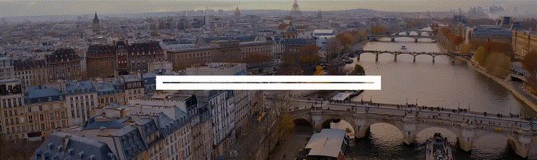
Application to artifical climbing walls in Paris and its neighbourhood

UAR RIATE, Université Paris Cité, CNRS

January 20, 2023

The aim of this notebook consists in showing how to build, visualize and reproduce accessibility indicators by combining points of interest (POI) coming from the OpenStreetMap database, socio-economic indicators included in small territorial division (IRIS) coming from institutional data source (INSEE) and routing engines (OSRM).

The graphical outputs displayed in this notebook are further developed in an Observable collection . To introduce the reader to the issues raised by indoor sport-climbing in Paris, have a look to this notebook .

This Quarto document combines 2 programming languages : R for data processing, and ObservableJS for data visualizations.

Data processing with R

The entire R script can be found here . Geojson files resulting from the data processing are available in the data-conso folder of the github repository of the project. These files are directly imported in Observable notebooks for data visualization.

Data sources

Three data sources, coming from three data providers, will be used:

IGN : The Contour…IRIS® édition 2020 , which corresponds to the lowest territorial division in France (below the communes level).

INSEE : for socio-economic indicators (IRIS Median income and population in 2019).

OpenStreetMap : download of Point Of Interest (POI) and travel time calculation by bike between IRIS centroids and POI, using the OSRM routing engine .

Input data is not provided in the GitHub repository (too large files), but can easily be downloaded and used (no constraints of use).

A bounding box of 5 km around Paris, without Bois de Boulogne and Bois de Vincennes for a better centering of the map layout around Paris is created.

A second bounding box (10 km around Paris) is created to catch OpenStreetMap POI and IRIS in the neighbourhood of this study area and avoid “border effects” for the upcoming travel-time indicators calculations.

Feed IRIS with socio-economic data (INSEE)

Data is enriched by socio-economic data (disposable median income 2019 and total population 2018) for further analysis. We keep only “Habitation” IRIS (dedicated to dwellings) for origins-destinations calculations.

Prepare IRIS for travel-time calculation

IRIS centroids are extracted. These points will be used for the origins of travel-time calculations. Only IRIS including dwellings are kept (TYP_IRIS == “H”).

These sf objects are transformed in latitude/longitude (origin-destination calculations requirements and for final export in geojson format).

Import OSM points of interest

Points of interest (climbing areas) are extracted from OpenStreetMap thanks to the osmdata R package ( Mark Padgham ( 2022 ) ).

To access to these OSM features, the OSM key-value pair (or OSM tag) must be set. For climbing areas, the most appropriate is sport=climbing . In the OpenStreetMap wiki , it is mentioned that “ sport=climbing should be preferably applied to noded for artificial climbing walls”. Thus, we only consider points responding to the query.

The geographical coverage of the query covers a bounding box of 10 km around Paris ( paris10k `).

The OSM attributes are transformed afterwards for further analytical purposes in order to differentiate private and associative structures, and bouldering areas and climbing walls (to different climbing practices).

I argue that the accuracy and completeness of the data is quite good : I have edited missing points on OpenStreetMap database with my personal knowledge and upstream investigation :-)

For the presentation of the artificial climbing landscape in Paris and the difference between private - FSGT and FFME structures, have a look to this notebook .

The data preparation allows to prepare origins-destinations layers for travel-time calculation. Origins correspond to the IRIS layer (only type H : 2141 points). Destinations to artificial climbing areas (45 points).

Travel-time calculations with OSRM

Origins and destinations required to compute travel-time calculations are now available. The computation is realized using the osrm R package ( Giraud ( 2022b ) ). This package allows the computation of routes, trips, isochrones and travel distances matrices (travel time and kilometer distance).

Considering that the input data are quite important (more than 2000 origin points and 48 destination points) and to avoid to overload the OSRM demo server, I have run my own instance of OSRM based on a docker container solution. The procedure to implement this solution is explained in the following documentation , or more specifically for Windows here .

Once it is done, the connection to the routing engine is operational locally (with the URL http://localhost:5000/ ` for me).

With OSRM, it is possible to choose several profiles depending on the routing we want to use (car, bike, walking). In our case, we choose the bike profile: Cycling is a widespread practice (with public transport) for climbers to reach their activities in this kind of urban context. Moreover, it allows also to avoid to use the car profile, which underestimates the travel-time in metropolitan areas (traffic congestion not taken into account).

The bicycle profile is described in the github OSRM repository . Basically, the default speed is 15 km/h. It avoids the access to highways, reduce the driving speed by 30 % for unsafe roads. It is important to keep in mind that landforms (elevation) are not considered in the default profile. Some thoughts and solutions exist on the subject, using elevation rasters ( Liedman (2022) ; Mapbox (2015) ). This will not be considered here.

IRIS to climbing areas

The code below compute travel-time calculation between the geometric centre of IRIS ( ori ) and artificial climbing areas ( dest ). It is done for all climbing structures and reproduced according to the type of climbing structure : private or associative structures. For associative structures, we distinguish the FSGT and FFME federations, that do not have exactly the same goals in term of practice.

Resulting travel-time matrixes are exported in the data-conso folder for other possible uses (and to avoid running these important calculations systematically).

This heavy matrix is then manipulated to extract for each IRIS the following information :

Name of the nearest climbing structure by bike.

Type of manager (private, FFME or FSGT).

Time to reach it (in minutes).

Number of artificial climbing areas at less than 15 minutes by bike (N).

This calculation is done for all climbing structures (ALL), for private ones (PRIV), for those held by FFME federation (FFME) and for those held by the FSGT federation (FSGT). It is done with R base code. A function would reduce considerably the code length… Nevermind, it is not the aim of the proof ;)

Characterizing the POI neighbourhood

Then, the socio-economic neighbourhood of each climbing area is characterized.

The previous matrix is transposed (lines <> columns). For each climbing structure, the IRIS located at less than 15 minutes by bike is extracted to produce the following indicators :

Total population at less than 15 minutes by bike. This can be considered as an amount of “local social demand”.

Minimum, mean and maximum of median income of IRIS at less than 15 minutes by bike.

Below is mapped one indicator calculated previously at IRIS level : time required to reach the nearest climbing area from the each populated IRIS centroid.

Travel time isochrones

Moreover, we can be interested by defining the accessibility of climbing areas without taking into account any territorial division, which can introduce numerous bias, due to MAUP effects. This is done by building isochrones of equivalent time-distance coming from climbing areas, using the mapiso R package ( Giraud ( 2022a ) ). Below are reminded the required steps to create polygons of equipotential from a regular grid of points :

• Create a regular grid (150m resolution in our case) and extract the centroids.
• Compute travel time indicators with the osrmtable function of the osrm R package, from grid centroids to climbing areas.
• Get the minimum value of the resulting matrix and join the result to the regular grid layer.
• Create polygons with mapiso function, wich takes the resulting values included in the regular grid. The function takes the desired thresholds and the indicator we are interested in (which climbing area travel time).

The maps below display the location of the climbing areas in the study area (white dots), the travel-time by bike required to reach each points from the 150m regular grid (dot map) and the resulting isochrones deducted from these values.

OSRM climbing trip

osrmTrip is a function from the osrm package ( Giraud ( 2022b ) ) which allows to get the travel geometry between multiple unordered points. The output is a sf LINESTRING with 2 components : duration (in minutes) and distance (in kilometres).

This function is applied to the climbing areas held by the FSGT federation.

To reach the 22 climbing areas of the FSGT federation located in the study area, the osrmTrip function returns that the fastest cycling trip around these climbing areas can be done in 420.93 minutes and 88.3846 kilometres.

Manual corrections (out of OSM)

I noticed that in the OpenStreetMap database some attributes could be specified more precisely. However, my use does not correspond to the one recommended by OSM : climbing_length is not climbing_max. Moreover, this attribute has been set directly in OSM by the private brand.

Consequently, I prefer not to change these attributes in the OSM database, but directly in my R programme.

Simplify geometries

Geometries are quite detailed. The library rmapshaper ( Andy Teucher ( 2022 ) ) is used to simplify the layer. 9 % of the points constituting the polygons are kept. Then, the IRIS layer is aggregated in communes for the map layout.

We also extract the IRIS located at less than 15 minutes from a artificial climbing area for some upcoming maps.

Export results

Data preparation is over. Resulting sf objects that will be used for data visualizations are exported in geojson files in the data-conso folder.

Session info (R)

Data visualization with observable javascript (ojs).

Observable is a startup founded by Mike Bostock and Melody Mechfessel, who initiated an on-line platform to collaboratively explore, analyse, visualize and communicate with data on the Web.

The computing language is Observable JavaScript (ojs) . It is possible to include this programming language in Quarto chunks.

This section imports some visualizations realized in an Observable collection . Have a look to this resource to see the overall project !

All the maps produced below use the bertin.js library ( Lambert ( 2023a ) ). Have a look to the documentation in this npm repository or in this Observable Collection to see the possibilities offered by this library to the map creator !

Import consolidated data

Geojson files coming from the data preparation precessing realized in a R programming language and described above are imported.

Bertin.js ( Lambert ( 2023a ) ), geotoolbox.js ( Lambert ( 2023b ) ) geoverview.js ( Lambert ( 2022 ) ) libraries are imported. These libraries will be used for creating the maps.

Layers attributes and metadata

Three geographical layers will be used :

• iris : IRIS intersecting the study area (polygons layer).
• poi : climbing structures included the study area (points layer).
• com : Municipalities intersecting the study area (polygons layer). This layer will only be used for the map layout and better understand the location of the poi and iris layers : IRIS, the lowest territorial division in France, is not really known by the population.

The first two geographical layers include attributes coming from the data preparation process, that will be mapped and plotted in the next section of the document. In this part, we present the layers in several ways to understand the information we have in hand for producing the data visualization.

Interactive map

Made with geoverview library. Click on the points / polygons to have an overview of their respective attributes and values.

Attributes and metadata

Attribute table (iris layer)

Indicators definition (iris layer)

Attribute table (poi layer)

Indicators definition (poi layer)

Wall’s characteristics

This interactive map displays the artificial climbing offer in Paris and its surroundings, according artificial climbing specificities: top rope climbing (walls) / bouldering, climbing height, number of routes, manager of the artificial climbing area.

Nearest wall

The nearest climbing area by bike from each populated IRIS by wall manager: private or associative (FSGT or FFME).

Time to climb (IRIS)

It displays the time by bike required to reach the nearest climbing area, for all structures or by manager type and from each IRIS centroids.

Time to reach climbing areas (isochrones)

It shows with isochrones the area reachable from the network of climbing areas by bike in minutes. It is possible to see all climbing areas (default map) or filter by manager (private or FSGT).

Climbing in 15 minutes?

The number of climbing areas reachable in 15 minutes by bike from the geometric centroid of each IRIS of the study area.

Climbing / biking tour !

It shows the fastest path to visit all the FSGT’s climbing areas by bike. To overcome this challenge, you will have to cycle for 88.39 km and 7.02 hours !

Demographic neighbourhood

Visualize the demographic neighbourhood of each climbing area : IRIS population at less than 15 minutes by bike from each climbing area.

Income neighbourhood

Visualize the level of wealth of each climbing area neighbourhood : IRIS median income at less than 15 minutes by bike from a climbing area. User can choose the minimum income, average income or maximum income of the IRIS at less than 15 minutes.

Concluding methodological remarks

Extend the analysis.

This methodological example showed a general methodology to combine institutional and crowd-sourced data to develop some simple indicators of accessibility to services of interest using open-source routing engines, and disseminate this with data visualizations frameworks. It is one possible implementation, among others. Other implementations could easily be envisaged, such as:

• Geographical coverage : The data preparation process presented above requires the definition of a geographical bounding box to extract OpenStreetMap points of interest (destinations of travel-time calculations) and an existing territorial division (the centroids being the origins of the travel-time calculations). This could be easily extended to other areas of interest, by modifying the Xmin, Xmax, Ymin and Ymax of the bounding box, or using other territorial divisions (a regular grid, for instance). The important things to consider is
• Use other points of interest : This example used the OpenStreetMap tag defined by the key-value sport=climbing . Other map features could be investigated, such as amenities , tourism facilities or shops . The only element to consider is the geometric reference of the object in the OpenStreetMap database ; it could be nodes, ways or relations. In the case of sport=climbing tag, the OpenStreetMap Wiki reminds that sport=climbing should preferably applied to nodes for artificial climbing walls , our case. If the tag combines nodes and areas, it requires also to extract polygons responding to the tag and transform it into points, checking if the information is not included twice in the OpenStreetMap database.
• Apply other profiles : In this example, the standard bike profile has been applied. The pedestrian and the car profile are also available and may be also used depending on the objective of the analysis. Whatever the profile used, it reminds important to the parameters of the profiles ( car here , bike here and pedestrian here ) to understand the calculations realized with routing engines, and their limitations. It is also possible to implement its own profile .

Usage precautions

One persisting criticism made to OpenStreetMap is its lack of quality, mainly due to its collaborative aspect implying de facto a high heterogeneity of contribution practices. Known problems refer to geometric accuracy (geographical positioning of OSM objects), accuracy , completeness (missing points, not up-to-date) or problems due to the tags describing OSM objects (missing important tags, bad practices).

In that case, I made a personal survey to complete missing information (around 30 % of the information was missing) in OpenStreetMap database. It meant add some missing points in some cases, and in others to describe it with relevant climbing tags identified in the OpenStreetMap Wiki. At the end, it is sure that the input information is not perfect and would require double-checks by the community, but we can argue that it was not worst than in the beginning.

Whatever the use of OpenStreetMap you may made, taking a step back to these questions is very important to control a minima the input information used for the travel-time calculations .

Another point to have in mind is the default parameters of osrm profiles: bike profile does not take into account the slope of the road ; the car profile does not take into account the traffic congestion. It may have significant impact on the travel-time calculations.

Nevertheless, we argue that OpenStreetMap is a wonderful initiative and as we try to demonstrate in this notebook, it is not too difficult to produce innovative indicators and data visualizations using open-source database and libraries.

Source Code

What is TravelTime?

Create a Travel Time Map

Travel time map generator & isochrones, i know i can get from a to b by public transport within my selected time, but it's not showing up.

• Walking to the station platform
• Waiting for the next available departure
• Time spent boarding the train
• Giving enough time to take the A to B journey
• Depart on the station on the other side.

You can't drive that far / you can drive much further than that"

• Open another mapping app of your choice and enter an A to B route
• Select a departure time for tomorrow.

Still not convinced?

About this tool, what is a travel time map, how to create a drive time radius map or other modes.

• Select a start location
• Select a maximum travel time limit
• Select a mode of transport, for example driving
• Voila! There's your driving radius map

Use cases for consumers

• Create a commute time map so you can see where to live based on commute time.
• How far can i travel in a given time: compare transport coverage for different areas.
• Create a drive time radius map: explore how far you can travel on a road trip.

Use cases for businesses

• Travel time mapping up to 4 hours & cross reference other data sets in GIS such as population data
• Site selection analysis: analyse the best location to locate a business by adding thousands of analysis points
• Create a distance matrix or travel time matrix & calculate travel times from thousands of origins to thousands of destinations
• Network analysis / travelling salesman problem: use spatial analytics to solve routing problems
• Commute time map - plot thousands of employee commute times for an office relocation
• Create up to 3 time polygons visualising where's reachable within 2 hours or less. Our API can create large travel time areas, talk to sales.
• Calculate travel times from an origin to various points of interest - in this demo we use points from Foursquare Give A to B routing details

Full access

• Book a demo
• Trial TravelTime API
• Trial QGIS Plugin
• Trial ArcGIS Pro Add-In
• Trial Alteryx Macros

TravelTime Features

• See 'How far can I get' in X minutes
• Create a drive time map or any other transport mode
• Overlap many shapes & highlight overlap area
• Search points of interest within the area
• Get A to B routing details

Developer Tools

Database Plugins

Isochrone API

Distance Map API

v4/distance-map

Travel Time Matrix API

Geocoding API

/v4/geocoding

Additional API Reference

Error Handling

About the plugin

Quick tools

Toolbox tools

About the macros

Travel Time R SDK

Travel Time R SDK helps users find locations by journey time rather than using ‘as the crow flies’ distance. Time-based searching gives users more opportunities for personalisation and delivers a more relevant search.

Installation

You can install Travel Time R SDK hosted on CRAN repository with the following command:

System requirements

traveltimeR uses rprotobuf as a dependency. If your package installation fails, please make sure you have the system requirements covered for rprotobuf

Debian/Ubuntu

There also exists similar commands on other distributions or operating systems.

Authentication

In order to authenticate with Travel Time API, you will have to supply the Application ID and API Key.

Isochrones (Time Map)

Given origin coordinates, find shapes of zones reachable within corresponding travel time. Find unions/intersections between different searches.

Isochrones (Time Map) Fast

A very fast version of Isochrone API. However, the request parameters are much more limited.

Distance Map

Given origin coordinates, find shapes of zones reachable within corresponding travel distance. Find unions/intersections between different searches.

Distance Matrix (Time Filter)

Given origin and destination points filter out points that cannot be reached within specified time limit. Find out travel times, distances and costs between an origin and up to 2,000 destination points.

Body attributes:

• locations: Locations to use. Each location requires an id and lat/lng values.
• departure_searches: Searches based on departure times. Leave departure location at no earlier than given time. You can define a maximum of 10 searches.
• arrival_searches: Searches based on arrival times. Arrive at destination location at no later than given time. You can define a maximum of 10 searches.

Returns routing information between source and destinations.

Time Filter (Fast)

A very fast version of time_filter() . However, the request parameters are much more limited.

Time Filter Fast (Proto)

A fast version of time filter communicating using protocol buffers .

The request parameters are much more limited and only travel time is returned. In addition, the results are only approximately correct (95% of the results are guaranteed to be within 5% of the routes returned by regular time filter).

This inflexibility comes with a benefit of faster response times (Over 5x faster compared to regular time filter) and larger limits on the amount of destination points.

• departureLat: Origin point latitude.
• departureLng: Origin point longitude.
• destinationCoordinates: Destination points. Cannot be more than 200,000.
• transportation: Transportation type.
• travelTime: Time limit.
• country: Return the results that are within the specified country.

Time Filter (Postcode Districts)

Find reachable postcodes from origin (or to destination) and get statistics about such postcodes. Currently only supports United Kingdom.

Time Filter (Postcode Sectors)

Find sectors that have a certain coverage from origin (or to destination) and get statistics about postcodes within such sectors. Currently only supports United Kingdom.

Time Filter (Postcodes)

Geocoding (search).

Match a query string to geographic coordinates.

Function accepts the following parameters:

• query - A query to geocode. Can be an address, a postcode or a venue.
• within.country - Only return the results that are within the specified country or countries. If no results are found it will return the country itself. Optional. Format:ISO 3166-1 alpha-2 or alpha-3.
• format.exclude.country - Format the name field of the response to a well formatted, human-readable address of the location. Experimental. Optional.
• format.name - Exclude the country from the formatted name field (used only if format.name is equal true). Optional.
• bounds - Used to limit the results to a bounding box. Expecting a character vector with four floats, marking a south-east and north-west corners of a rectangle: min-latitude,min-longitude,max-latitude,max-longitude. e.g. bounds for Scandinavia c(54.16243,4.04297,71.18316,31.81641). Optional.

Reverse Geocoding

Attempt to match a latitude, longitude pair to an address.

• lat - Latitude of the point to reverse geocode.
• lng - lng Longitude of the point to reverse geocode.

Get information about currently supported countries.

Supported Locations

Find out what points are supported by the api.

2018 Primetime Emmy & James Beard Award Winner

R&K Insider

Join our newsletter to get exclusives on where our correspondents travel, what they eat, where they stay. Free to sign up.

A History of Moscow in 13 Dishes

Featured city guides.

Where are all the boulders? Everything you need to know about a visit to Boulder City

I find it interesting the places I travel where the names do not always make sense.

For instance, I once traveled through Boring, Oregon and when I asked a man for a good place to have lunch - he jumped up and down, “Dude, there is this awesome burger joint, it’s always rockin’."

I drove through Canada and Texas a few years back and was surprised no one had a French accent, and the folks there liked me, an American.

Another time, I cruised through Intercourse, Pennsylvania - I did not stop.

Does Boulder City have lots of boulders?

So, when Laureen and I visited Boulder City, Nevada, recently, I saw no boulders.

“Where’s the boulders?” I asked.

My lovely wife shook her head. “It’s named after Boulder Canyon, where Hoover Dam was built.”

I nodded. “Still, it would be nice to see some boulders since its name is Boulder City. Just one huge granite rock stuck in the middle of the main street, with a sign pointing to that igneous thingie that says, "Welcome to Boulder City.”

“Time for lunch and your meds,” Laureen commented.

And soon, we found ourselves at the Boulder Dam Brewery in the Boulder City Historic District. All was well with the day.

It was our two-hundredth wedding anniversary, and as a surprise, I booked a room at the historic Boulder Dam Hotel.

Laureen wanted Paris, France, and frowned when I suggested Perris, California.

So to Nevada, we went.

No gambling in Boulder City? You betcha'

Boulder City is only one of two cities in Nevada that does not allow gambling. The other is a town named Panaca - somewhere near the border of Utah.

What if I wanted to wager a month's salary on the spinning ball of Roulette?

According to the Boulder Dam Hotel concierge, “You’ll have to leave town to gamble. This city was one of the first planned town developments in the nation, and gambling was not one of the vices for the residents.”

It turns out that Boulder City was built on federal land and was, in fact, an experiment on how to lay out a city with everything that would be needed for the folks who would reside in the area. There would be paved roads, houses, grocery stores, churches, and everything else that would make up a wholesome community, excluding games of chance.

The Bureau of Reclamation headed the project, tasked with overseeing the construction of the Boulder Canyon Project, later known as Hoover Dam, along with six separate construction companies that had won the building contracts from the federal government. The project was too humongous for any one company to construct.

It was in December of 1928 that President Calvin Coolidge authorized the building of Boulder City to house all the workers needed for the massive and ambitious plans of creating a dam along the mighty Colorado River.

“We need a place for our laborers to rest after laboring all day in a gazillion degrees while hanging off sheer cliff faces,” it is rumored that President Coolidge stated to a flunky.

The flunky may have nodded in agreement. “Should there be gambling?”

“Brothels?” the flunky asked.

“No brothels for them or you,” the president said quickly, grabbing a pen and ensuring it was in the construction by-laws.

It seems when news of the huge dam project was floating around the area of Boulder Canyon, the smallwigs in Las Vegas wanted dam workers to reside in Las Vegas - this was before Bugsy Siegel and the mob had taken over Sin City - they would later be known as bigwigs. Las Vegas was just a small gambling locale in the middle of the desert, and the smallwigs thought having a large group of men with loads of cash in their pockets after working all day along the river might bring some more stability to the desert gambling mecca.

The government, later to be known as Big Brother, told the gambling folks from Las Vegas to keep their distance from the hard-working men building the dam in the canyon.

“Last thing we need is to have a man lose a month’s salary in one naughty night in Las Vegas and have him dangling from a rope high above the Colorado River,” one foreman may have uttered.

“He may become untethered and then really untethered,” another foreman may have commented.

So, Boulder City was built in two years, from 1931 to 1932 - very fast for a full-blown town, but then again, the Hoover Dam was completed two years earlier than expected—a solid work ethic in those roaring thirties.

All the seven main streets in the town were named after states through which the Colorado River runs: Wyoming, Colorado, Utah, New Mexico, Arizona, Nevada, and California. It was a lovely touch since these states were also where many workers had resided before moving to Boulder City to be employed for the dam project.

Boulder City has some marvelous views

As Laureen and I drove through this beautiful hilltop town overlooking the stilled waters of the Colorado River just north of the Hoover Dam, we marveled at the view from Denver Street. The story goes that it has the same view as back in 1932, with huge mountain vistas looking east toward Arizona with the startling blue waters of Lake Mead below. I wondered about that for a moment. Why wouldn’t it have the same view? What could have changed the landscape? An earthquake, a meteor impact, the Colorado River drying up, or perhaps Denver Street rerouted through the years.

These are the ponderings that keep me awake at night.

After the dam was completed in 1936, the hydroelectric power was delivered to Nevada and Southern California and turned over to the Los Angeles Bureau of Power and Light (later changed to the Los Angeles Department of Water and Power) and the California Edison Company.

The Feds controlled the entire region upon which Boulder City was built until 1958, when Congress approved the Boulder City Act, allowing the Bureau of Reclamation to turn over nearly 33 square miles to the newly enacted city government. In January of 1960, Boulder City was incorporated with huge fanfare from its many residents.

“About time,” one happy resident was heard shouting.

The Bureau of Reclamation kept control of all facilities needed to ensure the proper operation and maintenance of such a vital structure as the dam. And even the townsfolk realized the federal government always ran things much better and more efficiently than the local bureaucrats could (he typed with a wink).

The historic district is meant to meander and leisurely enjoy all the sights. There is a comfortable and quaint feeling while walking down the town streets, with buildings dating back to the dam's construction.

Downtown Boulder City full of art, history

The downtown district is registered on the National Register of Historic Places, with most buildings dating from 1931 to 1942. Only 40 or so were built after 1950, and since there are 514 buildings within the district, the entire area is a historical adventure for the tourist to take in and appreciate.

To highlight how life was in the early days of Boulder City, there is wonderfully crafted metal artwork seemingly every few yards down the main street.

A work created by artist Sutton Betti depicts men known as puddlers. These men smoothed cement with shovels after a pour, creating the shape of the dam.

Further down the street, a huge green metal frog by artist Kim Kori is blowing a kiss to visitors. Dozens of other uniquely created metal sculptures with descriptive plaques explain who the artist is and why such a piece was crafted.

The Boulder Dam Hotel, our abode away from home, was also added to the National Register of Historic Places in July of 1982. The hotel was a vision of Jim Webb, who believed Boulder City would need a hotty-totty sort of place where VIPs could stay.

Folks like Mr. and Mrs. Cornelius Vanderbilt, Jr., Will Rogers, the Maharaja and Maharani of Indore, India, as well as Dr. and Dr. John R. Beyer, and many such important people who needed a hotel with air conditioning, private baths, and a lavish wood-paneled lobby. And this hotel meets all those specifications.A marvelous museum, which depicts the early days of Boulder City and the construction of the Hoover Dam, is one of the main points to see within the hotel, which is visited by over 45,000 people annually.

There are modern touches here and there, with newer structures housing hotels, restaurants, breweries, and the like. Still, the overall feeling is one of stepping back in time to see how the ingenuity and perseverance of the human spirit changed this section of the Mojave Desert into a modern and welcoming destination for travelers.

John can be contacted at [email protected]

Information

https://www.bcnv.org and https://www.boulderdamhotel.com/

This article originally appeared on Salinas Californian: Where are all the boulders? Everything you need to know about a visit to Boulder City

• International edition
• Australia edition
• Europe edition

A local’s travel guide to Austin: what to eat, see and do in three days

Standout spots include food truck parks, honky-tonk hangouts and Lady Bird’s wildflower sanctuary

A ustin has become one of the most popular places in the US to move to, and also to visit. Droves of people descend on the city in March for the South by Southwest tech, film and music festival and in the fall for the Austin City Limits music festival. And Austin is one of the top five destinations in the US for bachelorette parties. Don’t let the bachelorettes scare you away, though. Austin is a great place to spend a few days, so long as you do it like a local.

My family and I moved to Austin 12 years ago, after living in New York for many years. I’ve also lived in Washington DC , the San Francisco Bay Area and Philadelphia. Austin has a feel all of its own: it has a world-class music scene, great food that now goes well beyond Tex-Mex and barbecue, Texas history and fun shopping and museums – all with less hassle than bigger cities in the US.

Here’s my guide to a long weekend there. In addition to picks for adults, I’ve included some recommendations for families that our kids (now teenagers) have loved through the years. And I’m vegetarian, so I’ve chosen some of the city’s best veggie eats options. Don’t worry, my meat-eating wife made sure that I included great barbecue choices, too.

Day 1: Pool party & pickles

Start your day with a walk or run on the trail at Town Lake (it’s officially labeled on maps as Lady Bird Lake, but locals refer to it as Town Lake). This 10-mile (16km) trail on both sides of a dammed portion of Texas’s Colorado River (a different Colorado River than the bigger and more famous one) is tree-shaded, beautiful and one of Austinites’ favorite places to exercise. If you have time, walk through Zilker Park, which is right next to the trail. If you have kids, go to the new and very fun playground at Butler Park, complete with a splash pad just up the path from the playground.

Austin was one of the cities that started the food truck scene in the US several decades ago, and now there are more than 2,000 food trucks in the city. Some are located in trailer parks that have multiple truck options and picnic table seating. After your morning at Town Lake and Zilker Park, have lunch at the Picnic food truck park, or the nearby original location of local favorite Chuy’s (the Tex-Mex chain is now expanding throughout the US). Other great lunch options include Green Mesquite and Carpenters Hall .

In the afternoon, go for a swim at Barton Springs Pool . Open year-round, this massive basin measures three acres and is fed by underground natural springs. It’s open throughout the day, and it’s free before 8am and after 9pm.

Head back to your hotel or Airbnb for a rest, and then get ready for dinner. Tonight is casual: barbecue at Terry Black’s , or if you’re vegan, the food truck Rollin Smoke for a fantastic vegan barbecue sandwich made with baby portobello mushrooms, spicy slaw, barbecue sauce and pickles. It’s my favorite vegan barbecue sandwich in Austin (who says you can’t have barbecue if you’re veggie?), and it’s located in a food truck park with beautiful old trees shading the tables. Rollin Smoke has very good meat options, too (I’m told).

If you have young children, head to Phil’s Icehouse . They have burgers and a full playground where the kids can play before or after dinner. Just don’t put them on the spinning flower after the meal. And be sure to get some ice-cream after dinner at Amy’s Ice Creams , a longtime favorite of Austinites. Amy’s is located next to Phil’s, and it’s so good we had an Amy’s truck serve dessert at our wedding.

After dinner, head out to see some music at one of Austin’s many local music venues. One of our favorites is the Continental Club . There’s a main club downstairs and the intimate Continental Gallery upstairs, where you can see local musicians in a cozy space. Other great venues include C-Boy’s and the new Moody Amphitheater . For full local music listings on any night, check the Austin Chronicle . And if it’s summer, look to see if Blues on the Green has a free concert that night. If you have kids, take them to the free Rock the Park concert series, produced by local radio station KUTX.

Day 2: Breakfast tacos, books & bats

Start your day back at the lake with a rowing workout that’s almost, but not quite, on the lake. Rō Fitness is a local studio that has outdoor rowing classes by the water. It’s way more fun than working out at an indoor studio.

You’ll need fuel after your workout. Grab a breakfast taco at Veracruz or Tacodeli or Tamale House East . Breakfast tacos are an Austin staple (they are to Austin as bagels are to New York), and all three of these places have delicious options.

Today is a shopping day. Start out at BookPeople , one of the greatest bookstores in the US. It’s locally owned and independent, but the size of a superstore. BookPeople also dares to take a stand on issues, including being one of two bookstores that recently sued Texas state officials over a newly passed book ban law. It has an excellent kids section, and organizes live readings by kids’ authors.

After you’ve gotten your book fix, head across the street to Waterloo Records , one of the best record stores in the US. Waterloo carries new and used vinyl, CDs and merchandise from rock to jazz to local Texas music. For more shopping options, head over to the stores along South Congress Avenue and South First Street (including Roadhouse Relics , a neon art store and gallery that is one of our favorites), and if you want to go thrifting, our teens say Austin Pets Alive Thrift and Texas Thrift are the best.

After all of the shopping, it’s time for lunch. If you’re near BookPeople and Waterloo, head over to Soup Peddler, a local place for homemade soups, smoothies and fantastic grilled cheese sandwiches (trivia: Soup Peddler got its name because the founder started out delivering homemade soup by bike before opening full store locations). Or if you’re near South Congress and South First, go to the food trucks on South First or Underdog or Fresa’s .

As you’re heading back to rest up, grab an ice-cream at Amy’s, a gelato at Dolce Neve or cupcakes at Sugar Mama’s .

Some good dinner options for tonight include Loro , Suerte or Este . And if you’re looking for a vegetarian option, one of my favorite veggie restaurants is Bouldin Creek Cafe . It’s casual, with a great menu that includes vegan chips and queso. If it’s nice out, take a seat on the patio.

Tonight’s activity could be going to see the bats at the Congress Street Bridge. Austin has the largest urban bat colony in North America, and in season they live in one of the bridges that crosses the Colorado River (they migrate to Mexico in the cooler weather). Bat-watching is a lot more fun than you might imagine from horror movies (and these bats look more like birds than vampire bats). If you’re not in the mood for bats, head to the legendary Broken Spoke . Get there early for dance lessons, then hoof it at this classic Texas honky-tonk.

Day 3: Live oaks & Lady Bird wildflowers

It’s your last day in Austin, and it’s a good one for visiting a museum. Some of our favorites include the Bullock Museum to learn all about the history of our state (bonus fact: Texas was once its own country , and some people want it to be its own country again ). If you’re a fan of 1960s history, visit the excellent LBJ Presidential Library , which is the home of the 36th president’s papers. It has good exhibits on the US civil rights movement and 1960s US history in general. Another excellent museum option is the Blanton Museum of Art , or you could tour the Texas capitol (Austin is, after all, the capital of Texas). If you’re a nature fan, head to the Lady Bird Johnson Wildflower Center . And if you have kids, the Thinkery is an excellent children’s museum.

For lunch, it’s time for more barbecue (you’re in Austin, don’t fight it). Two terrific barbecue trucks are Mickelthwait and LeRoy and Lewis . And LeRoy and Lewis has another of my favorite vegetarian barbecue options: cauliflower burnt ends.

In the afternoon, head back to Town Lake. This time, get out on the water by renting a kayak, stand up paddleboard or paddle boat (a kid-friendly option). If you have time and energy for a drink, head over to the ABGB for happy hour. They have a great beer selection, lots of outdoor seating and local bands playing music.

For your farewell dinner, a few of our favorite restaurants that are a bit on the fancier end are Hestia , Uchi or the Lenoir wine garden, where dinner is served under live oak trees more than a hundred years old. And for a fantastic vegan option, go to Fabrik for a seven-course vegan tasting menu. You’ll need a reservation well in advance (they’re currently booking four to six weeks out). And for your final night in Austin, head out to another music venue. Or if you have kids, take them to the Austin favorite Peter Pan Mini Golf , which has been around for 75 years, or check Do512 Family for family events that are happening the dates you’re in town.

Question Time

When is the best time of year to visit austin.

There’s no dispute: it’s hot in the summer in Austin . A great time to visit is between October and May. From June through September, many days will be over 100F. If you’re here in the summer, spend lots of time at the Barton Springs pool.

Is Austin expensive?

Austin hotels can be expensive during big events like South by Southwest or the Formula One weekend. But for most dates, it’s less expensive than larger cities like New York, Los Angeles and San Francisco.

Will I need a car to get around Austin?

Most of the places that I’ve recommended are within walking distance from downtown. You can also rent bikes and scooters to get around. Austin’s public transportation is primarily through local buses, which can take you further out if needed. And car-share options are easy as well.

Steve Sachs is managing director of the Guardian US. He has worked at large and startup media companies for more than 20 years. He loves all kinds of music, and his most recent favorite concert, the Texas Songwriters Hall of Fame Show, featured a host of singer-songwriters including Lyle Lovett and Emmylou Harris

• Hometown tour

Most viewed

Amazon to launch drone delivery in metro Phoenix. Here's how it works and how to sign up

The future of unmanned delivery services is closer than it may seem — and it’s right in one of Arizona’s backyards.  

Tolleson, a small city about 11 miles west of Phoenix, will serve as the third home base for Amazon’s experimental drone project , the delivery service powerhouse announced in a news release on Monday.  

"When you're a small town in the middle of an urban landscape surrounded by major buildings and major cities, it's always cool when you can be the partner on something so grand," Tolleson Mayor Juan Rodriguez said. 

Arizona is no stranger to drone delivery, between Walmart and companies like FlyBy Robotics , but here's what you need to know about Amazon's program.

When is Amazon beginning drone delivery in Arizona? 

No specific date or month has been set for the drone delivery to launch, according to the news release. However, Amazon noted that drone deliveries will start in the West Valley in Tolleson.  

Amazon is still coordinating with the Federal Aviation Administration and Tolleson officials to ensure everything is in place for the program to commence.  

Where will drone deliveries come from?  

Amazon has already established several same-day delivery sites across the Valley, and the drones will be situated near Tolleson’s site during the experimental period.  

“These smaller sites are hybrid — part fulfillment center, part delivery station,” Amazon’s news release noted. “They allow us to fulfill, sort, and deliver products all from one site so we can get packages out to our customers even quicker.” 

Chick-fil-A via drone delivery? How the fight for sky dominance is heating up

Where in metro Phoenix can I receive Amazon drone deliveries? 

Once the program is clear to start, it will only operate within a 7-mile radius of the distribution center, Mayor Rodriguez told The Arizona Republic. Some west Phoenix and Avondale residents will be able to receive drone deliveries. 

Which cities have Amazon drone delivery?

Amazon first implemented this program in College Station, Texas, and Lockeford, California, in 2022. The Lockeford location will be closing, the news release said, promising more drone delivery locales in 2025. The College Station site will remain open.  

What time of day will drone deliveries be available?

Amazon uses drone delivery from 9:30 a.m. to 5 p.m. Sunday through Thursday in California, and 9:30 a.m.-5 p.m., seven days a week in College Station, Texas, Amazon said on its website . However, drone delivery isn't available during certain weather conditions.

How do I sign up for Amazon drone delivery?

West Valley residents can register for drone delivery by inputting their email address into a form . Interested parties will be contacted as FAA processes move forward, according to Amazon.

Current operations in College Station require participants to prepare their yard, have an Amazon employee survey your yard and install a marker prior to their first drone delivery.

After that, users can identify products available for drone delivery and select "today: within one hour" as the delivery option in check out. Then place the QR code delivery marker on the mini marker in your yard. Users than receive an email confirming the purchase and estimated time of the drone's arrival.

What's new with Amazon's drone delivery program? 

New drones, capable of flying in more weather conditions and carrying up to five pounds at a time, will be introduced in Tolleson.  

Amazon reported that these MK30 drones will be operative in Italy and the United Kingdom soon, but no timeline was available at the time of publication.  

How much weight can an Amazon drone carry?

Amazon is debuting new drones that can carry up to five pounds at a time. The drones were set to operate in Europe soon, though the company did not specify when they would launch.

U.S. tourist faces 12 years in prison after taking ammunition to Turks and Caicos

An Oklahoma man faces up to 12 years in prison on a Caribbean island after customs officials found ammunition in his luggage.

Ryan Watson traveled to Turks and Caicos with his wife, Valerie, to celebrate his 40th birthday on April 7. They went with two friends who had also turned 40.

The vacation came to an abrupt end when airport staff members found a zip-close bag containing bullets in the couple's carry-on luggage. Watson said it was hunting ammunition he had accidentally brought with him — but under a strict law in Turks and Caicos, a court may still impose a mandatory 12-year sentence.

"They were hunting ammunition rounds that I use for whitetail deer," Watson told NBC Boston in an interview conducted last week that aired after their first court appearance Tuesday.

"I recognized them, and I thought, 'Oh, man, what a bonehead mistake that I had no idea that those were in there,'" he said.

The couple were arrested and charged with possession of ammunition. Authorities seized their passports and explained the penalties they faced.

Valerie Watson said in the interview: "When I heard that, I immediately was terrified, because I was like we can't both be in prison for 12 years. We have kids at home, and this is such an innocent mistake."

The charges against her were dropped, and she returned home to Oklahoma City on Tuesday after the court hearing to be reunited with her two young children.

"Our goal is to get Ryan home, because we can’t be a family without Dad," she said.

The couple also spoke about the financial burden of a much longer-than-planned trip. "This is something that we may never recover from," Ryan Watson said.

The U.S. Embassy in the Bahamas issued a warning to travelers in September about a law that strongly prohibits possession of firearms or ammunition in Turks and Caicos, an overseas British territory southeast of the Bahamas that is a popular vacation spot.

It said: "We wish to remind all travelers that declaring a weapon in your luggage with an airline carrier does not grant permission to bring the weapon into TCI [Turks and Caicos Islands] and will result in your arrest."

The embassy added: "If you bring a firearm or ammunition into TCI, we will not be able to secure your release from custody."

The embassy and the government in Turks and Caicos did not immediately respond to requests for comment.

The same thing happened to another American, Bryan Hagerich, of Pennsylvania, who was arrested after ammunition was found in his luggage before he tried to board a flight out of Turks and Caicos in February. He said he accidentally left it in his bag.

Hagerich was on a family vacation with his wife and two young children but has now been in the country for 70 days. He spent eight days in prison before he posted bail.

"It’s incredibly scary. You know, you just don’t know what the next day may bring — you know, what path this may take," Hagerich told NBC Boston.

"You know, it’s certainly a lot different than packing your bags and going away with your family for a few days. It’s been the worst 70 days of my life," he said.

Hagerich, once a professional baseball player, was drafted by the Florida Marlins in the MLB 2007 June amateur draft from the University of Delaware.

His case goes to trial May 3.

Patrick Smith is a London-based editor and reporter for NBC News Digital.

Saguaro National Park offers travelers an iconic slice of the Southwest

Get your camera ready for Saguaro National Park .

The park is home to the tallest cactus species in the country and a symbol of the Southwest, the saguaro, They’re particularly concentrated in the west district of the park, just outside Tuscon, Arizona.

“We like to call that one the Instagram side because you can literally go anywhere in the park, and there will be at least two or three dozen saguaros in the background of your photo,” said Cam Juárez, Community Engagement and Outreach coordinator and public information officer at the park.   

Here’s what else travelers will find at Saguaro, the latest national park in USA TODAY’s yearlong series .

Why is Saguaro National Park worth seeing?

“Saguaros are super special because they only exist in this part of the world the way they do,” said Juárez. “You can visit certain parts of Mexico, you can visit certain parts of central Arizona, but you’re never going to see them the way you see them here.”

They’re not the only scenic beauties in the biodiverse park. 

“Our peaks are in the neighborhood of around 9,000 feet,” Juárez said. Visitors can find aspen, pine and fir trees in its sky islands. “As you climb every few 100 feet down in elevation, you're experiencing different biomes all the way down to grasslands, to desert shrub, to basically just what you would imagine a desert to look like.”

Which side is better for Saguaro National Park?

The park is divided into east and west districts, which bookend Tucson. Tucson International is the closest airport.

“My favorite is the west district, just because I love seeing the saguaro. You're going to have 2 million, versus maybe a quarter million saguaros on the east side,” Juárez said. “But if you're a backcountry hiker and you want to hike long distances, the east district, Rincon Mountain District, is definitely better.” 

He noted the Arizona Trail , from the U.S.-Mexico border up to the Grand Canyon, goes right through the east district. 

Can I drive in Saguaro National Park?

Yes. There is a $25 vehicle entry fee for the park, which is cashless. 

Visitors can purchase passes online at Recreation.gov or at a park kiosk using a debit or credit card.

How long does it take to go through Saguaro National Park?

You could visit both sides of the park in one day but may be better off with two.

“If you only have one day, definitely take the Cactus Forest loop ,” Juárez recommended. Cactus Forest Drive is a scenic 8-mile roadway in the east district. The west district has a 5-mile Bajada Loop Drive.

What is the best time to visit Saguaro National Park?

Juárez called October and mid-November magical. That’s just before the park’s busiest time of year, which he said runs from after Thanksgiving through April.

“Two times a year, we see a lot of rainstorms,” he added. “We have our traditional summer monsoons, and we have our winter rains. As a bimodal desert, you're going to see different blossoms at different times of the year.”

He said monsoons amplify the park’s already magnificent sunsets.

“The different colors of red and yellows and golds, coupled with purple skies, it's just everything that you see on postcards,” he said. “It just comes alive.”

What does the saguaro mean to Native Americans?

“The Tohono O’odham have a very special relationship with the park. Their whole culture revolves around the saguaro cactus, or as they call it, the Ha:san ,” Juárez said. Tribal members may harvest the fruit for traditional uses with a special permit through the Interior Department and National Park Service. “The fruit is harvested as part of their traditional medicine, their traditional foods. A lot of ceremonial wines come from that.”

He said other tribes tied to the land include Pascua Yaqui Tribe and Gila River Indian Community .

What else should visitors know about Saguaro?

“I would love for people to know that Saguaro National Park is making a concerted effort to be conscientious of the fact that the representation matters,” Juárez said. “ Friends of Saguaro National Park , in conjunction with our team here, developed what's called the Next Generation Ranger program, and it's not just a paid internship. It's an opportunity for (interns) to gain experience and gain what's called the Public Land Corps credit opportunity, which will help us diversify not just race and ethnicity but also ability and gender …  so when you walk into Saguaro National Park, you're going to run into very knowledgeable, very experienced, diverse young people that are matching our country's identity.”

Nearly 45% of the Tucson population is of Hispanic or Latino heritage, according to the U.S. Census . Several park staffers speak Spanish, including Juárez. 

“It comes in handy because we're not just talking our friends to the south. We're talking all the way down to Central America and South America that are visiting national parks,” he said, adding that sometimes they’ll welcome visitors in Spanish. “You should see the look on people's faces. They're like, ‘Wow, you speak my language.’ I encourage all of my coworkers and staff people to make it a point to try to at least learn how to say welcome and hello in different languages.”

National parks for every body: How to make the outdoors more accessible

The park is also making a concerted effort to welcome guests of all abilities. Both districts offer a variety of accommodations, including accessible trails , braille and large-text versions of the park brochure, touchable exhibits, captioned programs and more.

“I definitely am an active voice, as a person with a physical disability, that says we can't just give folks a smidgen of what able-bodied individuals can get,” Juárez said. “We should make a very concerted effort to expand on everything we've done so far.”

• Get started
• Accessibility
• Trip planning with detailed_itineraries()
• FAQ - Frequently Asked Questions
• Accounting for monetary costs
• Trade-offs between travel time and monetary cost
• Using the time_window parameter
• Travel time matrices

Calculate travel time matrix between origin destination pairs

Fast computation of travel time estimates between one or multiple origin destination pairs.

An object to connect with the R5 routing engine, created with setup_r5() .

Either a POINT sf object with WGS84 CRS, or a data.frame containing the columns id , lon and lat .

A character vector. The transport modes allowed for access, transfer and vehicle legs of the trips. Defaults to WALK . Please see details for other options.

A character vector. The transport mode used after egress from the last public transport. It can be either WALK , BICYCLE or CAR . Defaults to WALK . Ignored when public transport is not used.

A POSIXct object. Please note that the departure time only influences public transport legs. When working with public transport networks, please check the calendar.txt within your GTFS feeds for valid dates. Please see details for further information on how datetimes are parsed.

An integer. The time window in minutes for which r5r will calculate multiple travel time matrices departing each minute. Defaults to 10 minutes. By default, the function returns the result based on median travel times, but the user can set the percentiles parameter to extract more results. Please read the time window vignette for more details on its usage vignette("time_window", package = "r5r")

An integer vector (max length of 5). Specifies the percentile to use when returning travel time estimates within the given time window. For example, if the 25th travel time percentile between A and B is 15 minutes, 25% of all trips taken between these points within the specified time window are shorter than 15 minutes. Defaults to 50, returning the median travel time. If a vector with length bigger than 1 is passed, the output contains an additional column for each percentile specifying the percentile travel time estimate. each estimate. Due to upstream restrictions, only 5 percentiles can be specified at a time. For more details, please see R5 documentation at https://docs.conveyal.com/analysis/methodology#accounting-for-variability .

A fare structure object, following the convention set in setup_fare_structure() . This object describes how transit fares should be calculated. Please see the fare structure vignette to understand how this object is structured: vignette("fare_structure", package = "r5r") .

A number. The maximum value that trips can cost when calculating the fastest journey between each origin and destination pair.

An integer. The maximum walking time (in minutes) to access and egress the transit network, to make transfers within the network or to complete walk-only trips. Defaults to no restrictions (numeric value of Inf ), as long as max_trip_duration is respected. When routing transit trips, the max time is considered separately for each leg (e.g. if you set max_walk_time to 15, you could get trips with an up to 15 minutes walk leg to reach transit and another up to 15 minutes walk leg to reach the destination after leaving transit. In walk-only trips, whenever max_walk_time differs from max_trip_duration , the lowest value is considered.

An integer. The maximum cycling time (in minutes) to access and egress the transit network, to make transfers within the network or to complete bicycle-only trips. Defaults to no restrictions (numeric value of Inf ), as long as max_trip_duration is respected. When routing transit trips, the max time is considered separately for each leg (e.g. if you set max_bike_time to 15, you could get trips with an up to 15 minutes cycle leg to reach transit and another up to 15 minutes cycle leg to reach the destination after leaving transit. In bicycle-only trips, whenever max_bike_time differs from max_trip_duration , the lowest value is considered.

An integer. The maximum driving time (in minutes) to access and egress the transit network. Defaults to no restrictions, as long as max_trip_duration is respected. The max time is considered separately for each leg (e.g. if you set max_car_time to 15 minutes, you could potentially drive up to 15 minutes to reach transit, and up to another 15 minutes to reach the destination after leaving transit). Defaults to Inf , no limit.

An integer. The maximum trip duration in minutes. Defaults to 120 minutes (2 hours).

A numeric. Average walk speed in km/h. Defaults to 3.6 km/h.

A numeric. Average cycling speed in km/h. Defaults to 12 km/h.

An integer. The maximum number of public transport rides allowed in the same trip. Defaults to 3.

An integer between 1 and 4. The maximum level of traffic stress that cyclists will tolerate. A value of 1 means cyclists will only travel through the quietest streets, while a value of 4 indicates cyclists can travel through any road. Defaults to 2. Please see details for more information.

An integer. The number of Monte Carlo draws to perform per time window minute when calculating travel time matrices and when estimating accessibility. Defaults to 5. This would mean 300 draws in a 60-minute time window, for example. This parameter only affects the results when the GTFS feeds contain a frequencies.txt table.

An integer. The number of threads to use when running the router in parallel. Defaults to use all available threads (Inf).

A logical. Whether to show R5 informative messages when running the function. Defaults to FALSE (please note that in such case R5 error messages are still shown). Setting verbose to TRUE shows detailed output, which can be useful for debugging issues not caught by r5r .

A logical. Whether to show a progress counter when running the router. Defaults to FALSE . Only works when verbose is set to FALSE , so the progress counter does not interfere with R5 's output messages. Setting progress to TRUE may impose a small penalty for computation efficiency, because the progress counter must be synchronized among all active threads.

Either NULL or a path to an existing directory. When not NULL (the default), the function will write one .csv file with the results for each origin in the specified directory. In such case, the function returns the path specified in this parameter. This parameter is particularly useful when running on memory-constrained settings because writing the results directly to disk prevents r5r from loading them to RAM memory.

A data.table with travel time estimates (in minutes) between origin and destination pairs. Pairs whose trips couldn't be completed within the maximum travel time and/or whose origin is too far from the street network are not returned in the data.table . If output_dir is not NULL , the function returns the path specified in that parameter, in which the .csv files containing the results are saved.

Transport modes

R5 allows for multiple combinations of transport modes. The options include:

Transit modes: TRAM , SUBWAY , RAIL , BUS , FERRY , CABLE_CAR , GONDOLA , FUNICULAR . The option TRANSIT automatically considers all public transport modes available.

Non transit modes: WALK , BICYCLE , CAR , BICYCLE_RENT , CAR_PARK .

Level of Traffic Stress (LTS)

When cycling is enabled in R5 (by passing the value BIKE to either mode or mode_egress ), setting max_lts will allow cycling only on streets with a given level of danger/stress. Setting max_lts to 1, for example, will allow cycling only on separated bicycle infrastructure or low-traffic streets and routing will revert to walking when traversing any links with LTS exceeding 1. Setting max_lts to 3 will allow cycling on links with LTS 1, 2 or 3. Routing also reverts to walking if the street segment is tagged as non-bikable in OSM (e.g. a staircase), independently of the specified max LTS.

The default methodology for assigning LTS values to network edges is based on commonly tagged attributes of OSM ways. See more info about LTS in the original documentation of R5 from Conveyal at https://docs.conveyal.com/learn-more/traffic-stress . In summary:

LTS 1 : Tolerable for children. This includes low-speed, low-volume streets, as well as those with separated bicycle facilities (such as parking-protected lanes or cycle tracks).

LTS 2 : Tolerable for the mainstream adult population. This includes streets where cyclists have dedicated lanes and only have to interact with traffic at formal crossing.

LTS 3 : Tolerable for "enthused and confident" cyclists. This includes streets which may involve close proximity to moderate- or high-speed vehicular traffic.

LTS 4 : Tolerable only for "strong and fearless" cyclists. This includes streets where cyclists are required to mix with moderate- to high-speed vehicular traffic.

For advanced users, you can provide custom LTS values by adding a tag <key = "lts"> to the osm.pbf file.

Datetime parsing

r5r ignores the timezone attribute of datetime objects when parsing dates and times, using the study area's timezone instead. For example, let's say you are running some calculations using Rio de Janeiro, Brazil, as your study area. The datetime as.POSIXct("13-05-2019 14:00:00", format = "%d-%m-%Y %H:%M:%S") will be parsed as May 13th, 2019, 14:00h in Rio's local time, as expected. But as.POSIXct("13-05-2019 14:00:00", format = "%d-%m-%Y %H:%M:%S", tz = "Europe/Paris") will also be parsed as the exact same date and time in Rio's local time, perhaps surprisingly, ignoring the timezone attribute.

Routing algorithm

The travel_time_matrix() , expanded_travel_time_matrix() and accessibility() functions use an R5 -specific extension to the RAPTOR routing algorithm (see Conway et al., 2017). This RAPTOR extension uses a systematic sample of one departure per minute over the time window set by the user in the 'time_window' parameter. A detailed description of base RAPTOR can be found in Delling et al (2015). However, whenever the user includes transit fares inputs to these functions, they automatically switch to use an R5 -specific extension to the McRAPTOR routing algorithm.

Conway, M. W., Byrd, A., & van der Linden, M. (2017). Evidence-based transit and land use sketch planning using interactive accessibility methods on combined schedule and headway-based networks. Transportation Research Record, 2653(1), 45-53. doi:10.3141/2653-06

Delling, D., Pajor, T., & Werneck, R. F. (2015). Round-based public transit routing. Transportation Science, 49(3), 591-604. doi:10.1287/trsc.2014.0534

Other routing: detailed_itineraries () , expanded_travel_time_matrix () , pareto_frontier ()

Screen Rant

Park min-young’s time travel k-drama perfectly flips her most famous role 6 years later.

Park Min-young’s latest TV role, Marry My Husband's Ji-won, perfectly flips her most famous character from one of the best K-dramas of all time.

• Marry My Husband flips Park Min-young's Secretary Kim role in a revenge-filled time travel story.
• Ji-won escaped an abusive marriage after going back in time and decided to focus on her professional career.
• Both shows involve second chances and reevaluating life priorities for the main characters.

Park Min-young’s character in the time travel K-drama Marry My Husband perfectly flipped her most famous role, Kim Mi-so from What’s Wrong With Secretary Kim . One of the most acclaimed actors of her generation, Park Min-young has starred in several successful shows. This includes hits like What’s Wrong With Secretary Kim and Forecasting Love and Weather , the former of which is widely considered one of the best K-dramas of all time . Following a two-year hiatus from Korean dramas, Park Min-young recently starred in Marry My Husband , which ran from January 1 to February 20, 2024.

While shows like Her Prive Life and Forecasting Love and Weather were very well received, What’s Wrong With Secretary Kim arguably remains Park Min-young’s most famous role six years later. Released in 2018, What’s Wrong With Secretary Kim featured Park Min-young as Kim Mi-so, a highly efficient secretary who was now reconsidering her priorities. The show also starred Park Seo-joon as Young-joon , Mi-so’s boss. There are some interesting parallels between Marry My Husband and What’s Wrong With Secretary Kim , especially when it comes to the differences between Park Min-young’s characters.

Park Min-young’s Marry My Husband Character Flips Her Secretary Kim Role

Kang ji-won has the opposite goal from kim mi-so.

In Marry My Husband , Park Min-young plays Kang Ji-won , who, at the start of the series, has been diagnosed with terminal cancer. On the same day she received her diagnosis, Ji-won found out her husband was cheating on her with her best friend. Not only that, but the two of them were counting the days for Ji-won to die so that they could get the insurance money. To accelerate things, Ji-won’s husband tried to kill her once she found out about his affair. While Ji-won did tie in this timeline, she instantly woke up 10 years in the past.

Mi-so’s story was not as tragic as Ji-won’s, yet both of these characters realized there was something wrong with their lives and decided it was time to change.

Ji-won was mysteriously given the chance to rebuild her life in Marry My Husband , after which she decided not only to plot her revenge against her soon-to-be-husband but also to ditch everything that was hurting her. Ji-won built new friendships, stopped caring about pleasing everyone, and focused on her professional career instead of living for her fiancé. Ji-won regained control of her life after leaving an abusive marriage as part of a toxic family that also included an abusive mother-in-law. Her character arc in the time travel K-drama was the opposite of what Mi-so went through in What’s Wrong With Secretary Kim .

In What’s Wrong With Secretary Kim , Park Min-young’s character is somewhat happy professionally but dreams of building a family and wants to focus more on her personal life. Secretary Kim had built an incredible reputation as the trustable, competent executive secretary of an important CEO, yet she was not fully happy. Mi-so was tired of being known as “Secretary Kim” and wanted to build a life outside of work. Mi-so’s story was not as tragic as Ji-won’s, yet both of these characters realized there was something wrong with their lives and decided it was time to change.

How Marry My Husband Is Different From What’s Wrong With Secretary Kim

Marry my husband was about ji-won finding her strength.

Marry My Husband and What’s Wrong With Secretary Kim play with some similar tropes , including but not limited to romance at the workplace. That said, they are very different shows with very different tones. Marry My Husband adds a supernatural element to a classic tale of revenge, with the time travel aspect of the story setting the narrative for Kang Ji-won’s journey. Most of the show is told from the perspective of Ji-won, allowing viewers to connect with her as her plan for revenge progresses. Most Marry My Husband characters are oblivious to Ji-won’s secret, except for her boss, Ji-hyuk.

Marry My Husband Ending Explained: Does Ji-won Find Happiness?

What’s Wrong With Secretary Kim , on the other hand, tells its story from the perspective of Park Min-young and Park Seo-joon’s characters . It becomes clear right from episode 1 that Secretary Kim and Young-joon have feelings for each other and might become a couple. From then on, the show explores how Mi-so’s decision to leave her job affects not only her life but also her boss’ life. Their pasts are slowly revealed as the show progresses, with audiences learning that their connection is deeper than anyone imagined. Compared to Marry My Husband ’s time travel plot , What’s Wrong With Secretary Kim is more grounded.

Marry My Husband & What’s Wrong With Secretary Kim Do Have Things In Common

Both k-dramas were about second chances.

Despite the differences between What’s Wrong With Secretary Kim ’s Mi-so and Marry My Husband ’s Ji-won, both shows are essentially about the same thing – second chances. Even though they were facing different challenges, these two characters were given a second chance in life and reconsidered their priorities. Ji-won’s tragedy led her to distance herself from all the toxic people in her life, which is why Marry My Husband was not only about revenge but also about fresh starts. Park Min-young’s character in What’s Wrong With Secretary Kim was in a relatively good place, yet she rightfully felt like she deserved more.

Stream Marry My Husband on Prime Video

Stream What's Wrong With Secretary Kim on Hulu

Marry My Husband